Worse than quantum physics

I’m still down the rabbithole of thinking way too much about quantum foundations and negative probabilities, and this time I came across an interesting analogy, which I will attempt to explain in this post and the next one. This should follow on nicely from my last post, where I talked about one of the most famous weird features of quantum physics, the violation of the Bell inequalities.

It’s not necessary to read all of that post to understand this one, but you will need to be somewhat familiar with the Bell inequalities (and the CHSH inequality in particular) from somewhere else. For the more technical parts, you’ll also need to know a little bit about Abramsky and Hardy’s logical Bell formulation, which I also covered in the last post. But the core idea probably makes some kind of sense without that background.

So, in that last post I talked about the CHSH inequality and how quantum physics violates the classical upper limit of 2. The example I went through in the post is designed to make the numbers easy, and reaches a value of 2.5, but it’s possible to pick a set of measurements that pushes it further again, to a maximum of (which is about 2.828). This value is known as the Tsirelson bound.

This maximum value is higher than anything allowed by classical physics, but doesn’t reach the absolute maximum that’s mathematically attainable. The CHSH inequality is normally written something like this:

Each of the s has to be between -1 and +1, so if it was possible to always measure +1 for the first three and -1 for the last one you’d get 4.

This kind of hypothetical ‘superquantum correlation’ is interesting because of the potential to illuminate what’s special about the Tsirelson bound – why does quantum mechanics break the classical limit, but not go all the way? So systems that are ‘worse than quantum physics’ and push all the way to 4 are studied as toy models that can hopefully illuminate something about the constraints on quantum mechanics. The standard example is known as the Popescu-Rohrlich (PR) box, introduced in this paper.

This sounds familiar…

I was reading up on the PR box a while back, and it reminded me of something else I looked into. In my blog posts on negative probability, I used a simple example due to Dan Piponi. This example has the same general structure as measurements on a qubit, but it’s also ‘worse than quantum mechanics’, in the sense that one of the probabilities is more negative than anything allowed in quantum mechanics. Qubits are somewhere in the middle, in between classical systems and the Piponi box.

I immediately noticed the similarity, but at first I thought it was probably something superficial and didn’t investigate further. But after learning about Abramsky and Hardy’s logical formulation of the Bell inequalities, which I covered in the last post, I realised that there was an exact analogy.

This is really interesting to me, because I had no idea that there was any sort of Tsirelson bound equivalent for a single particle system. I’ve already spent quite a bit of time in the last couple of years thinking about the phase space of a single qubit, because it seems to me that a lot of essential quantum weirdness is hidden in there already, before you even consider entanglement with a second qubit – you’ve already got the negative probabilities, after all. But I wasn’t expecting this other analogy to turn up.

I haven’t come across this result in the published literature. But I also haven’t done anything like a thorough search, and it’s quite difficult to because Piponi’s example is in a blog post, rather than a paper. So maybe it’s new, or maybe it’s too simple to write down and stuck in the ghost library, or maybe it’s all over the place and I just haven’t found it yet. I really don’t know, and it seemed like the easiest thing was to just write it up and then try and find out once I had something concrete to point at. I am convinced it hasn’t been written up at anything like a blog-post-style introductory level, so hopefully this can be useful however it turns out.

Post structure

I decided to split this argument into two shorter parts and post them separately, to make it more readable. This first part is just background on the Tsirelson bound and the PR box – there’s nothing new here, but it was useful for me to collect the background I need in one place. I also give a quick description of Piponi’s box model.

In the second post, I’ll move on to explaining the single qubit analogy. This is the interesting bit!

The Tsirelson bound: Mermin’s machine again

To illustrate how Tsirelson’s bound is attained, I’ll go back to Mermin’s machine from the last post. I’ll use the same basic setup as before, but move the settings on the detectors:

This time the two settings on each detector are at right angles to each other, and the right hand detector settings are rotated 45 degrees from the left hand detector. As before, quantum mechanics says that the probabilities of different combinations of lights flashing will obey

,

,

where is the angle between the detector settings. The numbers are more hassly than Mermin’s example, which was picked for simplicity – here’s the table of probabilities:

Then we follow the logical Bell procedure of the last post, take a set of mutually contradictory propositions (the highlighted cells) and find their combined probability. This gives , or, converting to expectation values ,

.

This is the Tsirelson bound.

The PR box

The idea of the PR box is to get the highest violation of the inequality possible, by shoving all of the probability into the highlighted cells, like this:

This time, adding up all the highlighted boxes gives the maximum .

Signalling

This is kind of an aside in the context of this post, but the original motivation for the PR box was to demonstrate that you could push past the quantum limit while still not allowing signalling between the two devices: if you only have access the left hand box, for example, you can’t learn anything about the right hand box’s dial setting. Say you set the left hand box to dial setting . If the right hand box was set to you’d end up measuring T with a probability of

.

If the right hand box was set to instead you’d still get :

.

The same conspiracy holds if you set the left hand box to , so whatever you do you can’t find out anything about the right hand box.

Negative probabilities

Another interesting feature of the PR box, which will be directly relevant here, is the connection to negative probabilities. Say you want to explain the results of the PR box in terms of underlying probabilities for all of the settings at once. This can’t be done in terms of normal probabilities, which is not surprising: this property of having consistent results independent of the measurement settings you choose is exactly what’s broken down for non-classical systems like the CHSH system and the PR box.

However you can reproduce the results if you allow some negative probabilities. In the case of the PR box, you end up with the following:

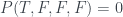
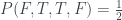
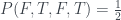
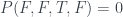
(I got these from Abramsky and Brandenburger’s An Operational Interpretation of Negative Probabilities and No-Signalling Models.) To get back the probabilities in the table above, sum up all relevant Ps for each dial setting. As an example, take the top left cell of the table above. To get the probability of (T,T) for dial setting (a,b), sum up all cases where a and b are both T:

In this way we recover the values of all the measurements in the table – it’s only the s that are negative, not anything we can actually measure. This feature, along with the way that the number crops up specifically, is what reminded me of Piponi’s blog post.

Piponi’s box model

The device in Piponi’s example is a single box containing two bits and , and you can make one of three measurements: the value of , the value of , or the value of . The result is either T or F, with probabilities that obey the following table:

These measurements are inconsistent and can’t be described with any normal probabilities , but, as with the PR box, they can with negative probabilities:

For example, the probability of measuring and getting F is

,

as in the table above.

Notice that crops up again! The similarities to the PR box go deeper, though. The PR box is a kind of extreme version of the CHSH state of two entangled qubits – same basic mathematics but pushing the correlations up higher. Analogously, Piponi’s box is an extreme version of the phase space for a single qubit. In both cases, quantum mechanics is perched intriguingly in the middle between classical mechanics and these extreme systems. I’ll go through the details of the analogy in the next post.