Bell’s theorem and Mermin’s machine

> Anybody who’s not bothered by Bell’s theorem has to have rocks in his head.

— ‘A distinguished Princeton physicist’, as told to David Mermin

This post is a long, idiosyncratic discussion of the Bell inequalities in quantum physics. There are plenty of good introductions already, so this is a bit of a weird thing to spend my time writing. But I wanted something very specific, and couldn’t find an existing version that had all the right pieces. So of course I had to spend far too much time making one.

My favourite introduction is Mermin’s wonderful Quantum Mysteries for Anyone. This is an absolute classic of clear explanation, and lots of modern pop science discussions derive from it. It’s been optimised for giving a really intense gut punch of NOTHING IN THE WORLD MAKES SENSE ANY MORE, which I’d argue is the main thing you want to get out of learning about the Bell inequalities.

However, at some point if you get serious you’ll want to actually calculate things, which means you’ll need to make the jump from Mermin’s version to the kind of exposition you see in a textbook. The most common modern version of the Bell inequalities you’ll see is the CHSH inequality, which looks like this:

(It doesn’t matter what all of that means, at the moment… I’ll get to that later.) The standard sort of derivations of this tend to involve a lot of fussing with algebraic rearrangements and integrals full of s and so forth. The final result is less of a gut punch and more of a diffuse feeling of unease: “well I guess this number has to be between -2 and 2, but it isn’t”.

This feels like a problem to me. There’s a 1929 New Yorker cartoon which depicts ordinary people in the street walking around dumbstruck by Einstein’s theory of general relativity. This is a comic idea because the theory was famously abstruse (particularly back then when good secondary explanations were thin on the ground). But the Bell inequalities are accessible to anyone with a very basic knowledge of maths, and weirder than anything in relativity. I genuinely think that everyone should be walking down the street clutching their heads in shock at the Bell inequalities, and a good introduction should help deliver you to this state. (If you don’t have rocks in your head, of course. In that case nothing will help you.)

It’s also a bit of an opaque black box. For example, why is there a minus sign in front of one of the s but not the others? I was in a discussion group a few years back with a bunch of postdocs and PhD students, all of us with a pretty strong interest in quantum foundations, and CHSH came up at some point. None of us had much of a gut sense for what that minus sign was doing… it was just something that turned up during some algebra.

I wanted to trace a path from Mermin’s explanation to the textbook one, in the hope of propagating some of that intuitive force forward. I wrote an early draft of the first part of this post for a newsletter in 2018 but couldn’t see how to make the rest of it work, so I dropped it. This time I had a lot more success using some ideas I learned in the meantime. I ended up taking a detour through a third type of explanation, the ‘logical Bell inequalities’ approach of Abramsky and Hardy. This is a general method that can be used on a number of other similar ‘no-go theorems’, not just Bell’s original. It gives a lot more insight into what’s actually going on (including that pesky minus sign). It’s also surprisingly straightforward: the main result is a few steps of propositional logic.

That bit of propositional logic is the most mathematically involved part of this post. The early part just requires some arithmetic and the willingness to follow what Mermin calls ‘a simple counting argument on the level of a newspaper braintwister’. No understanding of the mathematics of quantum theory is needed at all! That’s because I’m only talking about why the results of quantum theory are weird, and not how the calculations that produce those results are done.

If you also want to learn to do the calculations, starting from a basic knowledge of linear algebra and complex numbers, I really like Michael Nielsen and Andy Matuschak’s Quantum Country, which covers the basic principles of quantum mechanics and also the Bell inequalities. You’d need to do the ‘Quantum computing for the very curious’ part, which introduces a lot of background ideas, and then the ‘Quantum mechanics distilled’ part, which has the principles and the Bell stuff.

There’s also nothing about how the weirdness should be interpreted, because that is an enormous 90-year-old can of rotten worms and I would like to finish this post some time in my life

Mermin’s machine

So, on to Mermin’s explanation. I can’t really improve on it, and it would be a good idea to go and read that now instead, and come back to my version afterwards. I’ve repeated it here anyway though, partly for completeness and partly because I’ve changed some notation and other details to mesh better with the Abramsky and Hardy version I’ll come to later.

(Boring paragraph on exactly what I changed, skip if you don’t care: I’ve switched Mermin’s ‘red’ and ‘green’ to ‘true’ and ‘false’, and the dial settings from 1,2,3 on both sides to on the left side and on the right side. I’ve also made one slightly more substantive change. Mermin explains at the end of his paper that in his setup, ‘One detector flashes red or green according to whether the measured spin is along or opposite to the field; the other uses the opposite color convention’. I didn’t want to introduce the complication of having the two detectors with opposite wiring, and have made them both respond the same way, flashing T for along the field and F for opposite. But I also wanted to keep Mermin’s results. To do that I had to change the dial positions of the right hand dial, so that is opposite , is opposite , and is opposite . )

Anyway, Mermin introduces the following setup:

The machine in the middle is the source. It fires out some kind of particle – photons, electrons, frozen peas, whatever. We don’t really care how it works, we’ll just be looking at why the results are weird.

The two machines on the right and left side are detectors. Each detector has a dial with three settings. On the left they’re labelled , and . On the right, they’re , and .

On the top of each are two lights marked T and F for true and false. (Again, we don’t really care what’s true or false, we’re keeping everything at a kind of abstract, operational level and not going into the practical details. It’s just two possible results of a measurement.)

It’s vital to this experiment that the two detectors cannot communicate at all. If they can, there’s nothing weird about the results. So assume that a lot of work has gone into making absolutely sure that the detectors are definitely not sharing information in any way at all.

Now the experiment just consists of firing out pairs of particles, one to each detector, with the dials set to different values, and recording whether the lights flash red or green. So you get a big list of results of the form

The second important point, other than the detectors not being able to communicate, is that you have a free choice of setting the dials. You can set them both beforehand, or when the particles are both ‘in flight’, or even set the right hand dial after the left hand detector has already received its particle but before the right hand particle gets there. It doesn’t matter.

Now you do like a million billion runs of this experiment, enough to convince you that the results are not some weird statistical fluctuation, and analyse the results. You end up with the following table:

Each dial setting has a row, and the entries in that row give the probabilities for getting the different results. So for instance if you set the dials to and , there’s a 1/8 chance of getting (T,T).

This doesn’t obviously look particularly weird at first sight. It only turns out to be weird when you start analysing the results. Mermin condenses two results from this table which are enough to show the weirdness. The first is:

Result 1: This result relates to the cases where the two dials are set to , , or . In these cases both lights always flash the same colour. So you might get , , etc, but never or .

This is pretty easy to explain. The detectors can’t communicate, so if they do the same thing it must be something to do with the properties of the particles they are receiving. We can explain it straightforwardly by postulating that each particle has an internal state with three properties, one for each dial position. Each of these takes two possible values which we label T or F. We can write these states as e.g.

where the the entries on the top line refer to the left hand particle’s state when the dial is in the , and positions respectively, and the bottom line refers to the right hand particle’s state when the dial is in the , , position.

Result 1 implies that the states of the two particles must always be the same. So the state above is an allowed one, but e.g.

isn’t.

Mermin says:

> This hypothesis is the obvious way to account for what happens in [Result 1]. I cannot prove that it is the only way, but I challenge the reader, given the lack of connections between the devices, to suggest any other.

Because the second particle will always have the same state to the first one, I’ll save some typing and just write the first one out as a shorthand. So the first example state will just become TTF.

Now on to the second result. This one covers the remaining options for dial settings, , and the like.

Result 2: For the remaining states, the lights flash the same colour 1/4 of the time, and different colours 3/4 of the time.

This looks quite innocuous on first sight. It’s only when you start to consider how it meshes with Result 1 that things get weird.

(This is the part of the explanation that requires some thinking ‘on the level of a newspaper braintwister’. It’s fairly painless and will be over soon.)

Our explanation for result 1 is that particles in each run of the experiment have an underlying state, and both particles have the same state. Let’s go through the implications of this, starting with the example state TTF.

I’ve enumerated the various options for the dials in the table below. For example, if the left dial is and the right dial is , we know that the left detector will light up T and the right will light up T, so the two lights are the same.

Overall there’s a 1/3 chance of being the same and a 2/3 chance of being different. You can convince yourself that this is also true for all the states with two Ts and an F or vice versa: TTF TFF, TFT, FTT, FTF, FFT.

That leaves TTT and FFF as the other two options. In those cases the lights will flash the same colour no matter what the dial is set to.

So whatever the underlying state is, the chance of the two lights being different is greater than ⅓. But this is incompatible with Result 2, which says that the probability is ¼.

(The thinky part is now done.)

So Results 1 and 2 together are completely bizarre. No assignment of states will work. But this is exactly what happens in quantum mechanics!

You probably can’t do it with frozen peas, though. The details don’t matter for this post, but here’s a very brief description if you want it: the particles should be two spin-half particles prepared in a specific ‘singlet’ state, the dials should connect to magnets that can be oriented in three states at 120 degree angles from each other, and the lights on the detectors measure spin along and opposite to the field. The magnets should be set up so that the state for setting on the left hand side is oriented at 180 degrees from the state for setting on the right hand side; similarly should be opposite and opposite . I’ve drawn the dials on the machine to match this. Quantum mechanics then says that the probabilities of the different results are

where is the angle between the magnet states on the left and right sides. This reproduces the numbers in the table above.

Once more with less thinking

Mermin’s argument is clear and compelling. The only problem with it is that you have to do some thinking. There are clever details that apply to this particular case, and if you want to do another case you’ll have to do more thinking. Not good. This is where Abramsky and Hardy’s logical Bell approach comes in. It requires more upfront setup (so actually more thinking in the short term – this section title is kind of a lie, sorry) but can then be applied systematically to all kinds of problems.

This first involves reframing the entries in the probability table in terms of propositional logic. For example, we can write the result (T,F) for (a’,b) as . Then the entries of the table correspond to the probabilities we assign to each statement: in this case, .

Now, look at the following highlighted cells in three rows of the grid:

These correspond to the three propositions

,

which can be written more simply as

.

where the stands for logical equivalence. This also means that can be substituted for , and so on, which will be useful in a minute.

Next, look at the highlighted cells in these three rows:

These correspond to

,

which can be simplified to

.

where the stands for exclusive or.

Now it can be shown quite quickly that these six propositions are mutually contradictory. First use the first three propositions to get rid of , and , leaving

You can check that these are contradictory by drawing out the truth table, or maybe just by looking at them, or maybe by considering the following stupid dialogue for a while (this post is long and I have to entertain myself somehow):

Grumpy cook 1: You must have either beans or chips but not both.

Me: OK, I’ll have chips.

Grumpy cook 2: Yeah, and also you must have either beans or peas but not both.

Me: Fine, looks like I’m having chips and peas.

Grumpy cook 3: Yeah, and also you must have either chips or peas but not both.

Me: …

Me: OK let’s back up a bit. I’d better have beans instead of chips.

Grumpy cook 1: You must have either beans or chips but not both.

Me: I know. No chips. Just beans.

Grumpy cook 2: Yeah, and also you must have either beans or peas but not both.

Me: Well I’ve already got to have beans. But I can’t have them with chips or peas. Got anything else?

Grumpy cook 3: NO! And remember, you must have either chips or peas.

Me: hurls tray

So, yep, the six highlighted propositions are inconsistent. But this wouldn’t necessarily matter, as some of the propositions are only probabilistically true. So you could imagine that, if you carefully set some of them to false in the right ways in each run, you could avoid the contradiction. However, we saw with Mermin’s argument above that this doesn’t save the situation – the propositions have ‘too much probability in total’, in some sense, to allow you to do this. Abramsky and Hardy’s logical Bell inequalities will quantify this vague ‘too much probability in total’ idea.

Logical Bell inequalities

This bit involves a few lines of logical reasoning. We’ve got a set of propositions (six of them in this example case, in general), each with probability . Let be the probability of all of them happening together. Call this combined statement

.

Then

where the second equivalence is de Morgan’s law. This is definitely less than the sum of the probabilities of all the s:

.

where is the total number of propositions. Rearranging gives

.

Now suppose the are jointly contradictory, as in the Mermin example above, so that the combined probability . This gives the logical Bell inequality

.

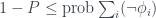
This is the precise version of the ‘too much probability’ idea. In the Mermin case, there are six propositions, three with probability 1 and three with probability ¾, which sum to 5.25. This is greater than , so the inequality is violated.

This inequality can be applied to lots of different setups, not just Mermin’s. Abramsky and Hardy use the CHSH inequality mentioned in the introduction to this post as their first example. This is probably the common example used to introduce Bell’s theorem, though the notation is usually somewhat different. I’ll go though Abramsky and Hardy’s version and then connect it back to the standard textbook notation.

The CHSH inequality

The CHSH experiment only uses two settings on each side, not three. I’ve drawn a ‘CHSH machine’ in the style of Mermin’s machine to illustrate it:

There are two settings and on the left side, 60 degrees apart. And there are two settings and on the right side, also 60 degrees apart, with opposite . This leads to the following table:

Now it’s just a case of following the same reasoning as for the Mermin case. The highlighted rows correspond to the propositions

As with Mermin’s example, these four propositions can be seen to be contradictory. Rather than trying to make up more stupid dialogues, I’ll just follow the method in the paper. First use to replace with in :

Then use to swap out again, this time with :

Finally use to swap out with , leaving

which is clearly contradictory.

(Sidenote: I guess these sort of arguments to show a contradiction do involve some thinking, which is what I was trying to avoid earlier. But in each case you could just draw out a truth table, which is a stupid method that a computer could do. So I think it’s reasonable to say that this is less thinking than Mermin’s method.)

Again, this violates the logical Bell inequality. In total, we have

.

The textbook version of this inequality is a bit different. For a start, it uses an ‘expectation value’ for each proposition rather than a straightforward probability, where truth is associated with +1 and falsity with -1. So each proposition has an expectation value with

Then summing over the s gives

and then, using the previous form of the logical Bell inequality,

.

A similar argument for shows that , so that this is a bound above and below:

.

In this case and so the inequality becomes . However adding up the s associated to the propositions gives 2.5, so the inequality is violated.

There’s still a little further to go to get the textbook version, but we’re getting close. The textbook version writes the CHSH inequality as

.

where the expectation value is written in the form

.

The are ‘hidden variables’ – properties of the particles that dispose them to act in various ways. For example, in the Mermin case, we imagined them to have hidden states, like

that controlled their response to each dial, and showed that any choice of these hidden states would lead to a contradiction.

For a given , and are the values measured by the left and right hand machines respectively. In our case these values are always either +1 (if the machine flashes T) or -1 (if the machine flashes F). The CHSH argument can also be adapted to a more realistic case where some experimental runs have no detection at all, and the outcome can also be 0, but this simple version won’t do that.

For the dial settings and , all we care about with these hidden variables is whether they make the machines respond true or false. So in our case is just a set of four variables, , and the integral can just become a sum:

.

.

Now that first proposition is just from earlier, which had probability . And the second one covers all the remaining possibilities, so it has probability . So

.

The argument goes through exactly the same way for and . The last case, , is slightly different. We get

following the same logic as before. But this time 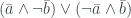matches the second proposition , not the first, so that

.

This is where the minus sign in the CHSH inequality comes in! We have

.

So we end up with the standard inequality, but with a bit more insight into where the pieces come from. Also, importantly, it’s easy to extend to other situations. For example, you could follow the same method with the six Mermin propositions from earlier to make a kind of ‘Mermin-CHSH inequality’:

.

Or you could have three particles, or a different set of measurements, or you could investigate what happens with other tables of correlations that don’t appear in quantum physics… this is a very versatile setup. The original paper has many more examples.

Final thoughts

There are still some loose ends that it would be good to tie up. I’d like to understand exactly how the inequality-shuffling in a ‘textbook-style’ proof of the CHSH inequality connects to Abramsky and Hardy’s version. Presumably some of it is replicating the same argument, but in a more opaque form. But also some of it must need to deal with the fact that it’s a more general setting, and includes things like measurements returning 0 as well as +1 or -1. It would be nice to figure out which bits are which. I think Bell’s original paper didn’t have the zero thing either, so that could be one place to look.

On the other hand… that all sounds a bit like work, and I can’t be bothered for now. I’d rather apply some of this to something interesting. My next post is probably going to make some connections between the logical Bell inequalities and my previous two posts on negative probability.

If you know the answers to my questions above and can save me some work, please let me know in the comments! Also, I’d really like to know if I’ve got something wrong. There are a lot of equations in this post and I’m sure to have cocked up at least one of them. More worryingly, I might have messed up some more conceptual points. If I’ve done that I’m even more keen to know!